Genealogy Beyond the Y
Chromosome
Autosomes Exposed
Stephen P. Morse
This article appeared in the Association of
Professional Genealogists Quarterly (March 2012).
This paper is a follow-up to a previous paper that I wrote entitled “From DNA to Genetic Genealogy: Everything you wanted to know but were afraid to ask,” published in two parts in the Association of Professional Genealogists Quarterly (March 2009 and September 2010). That paper described the use of DNA for learning about direct male ancestors and direct female ancestors. This paper deals with all your ancestors.
For the record, let me state that I am not a geneticist or a biologist or a chemist. Nor do I have any affiliation with a DNA testing laboratory. Rather I’m an engineer, with a personal interest in my own genealogy. I became involved in DNA because of the recent focus of DNA in genealogy. I realized that I didn’t have the background to understand how DNA was being used for genealogy because DNA was “invented” after I went to school. So I decided to teach myself about genes, chromosomes, and DNA. And in doing so, I developed a series of lectures on the subject. These papers are an outgrowth of those lectures.
1. INTRODUCTION
a. Genes, Chromosomes, and DNA
This will be a very abridged overview of the basic DNA concepts. For a more detailed description, see my original paper.
Everything we need to know about genetic genealogy involves three fundamental entities – genes, chromosomes, and DNA. The relationship between them is simple:
Traits are determined by GENES.
Genes are located on CHROMOSOMES.
Chromosomes are composed of DNA.
A chromosome is a long DNA molecule. The DNA structure is a double helix with the two strands running in opposite directions (see figure below). The direction of each strand is determined by its chemical composition, but we won’t say any more about the direction since it doesn’t affect the genealogy story.
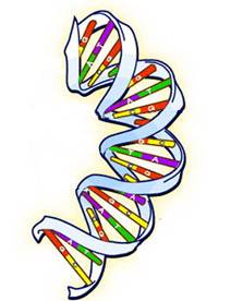
Each of the strands consists of four repeating compounds, which are called bases or nucleotides. The four bases are:
Adenine (A)
Cytosine (C)
Guanine (G)
Thymine (T)
Fortunately we don’t have to remember these names but can refer to them simply by their initials – A, C, G, T.
The bases on the two strands always pair up in a specific way. In particular, A on one strand always pairs with T on the other, and C always pairs with G. Why are there no other pairings, such as A with G? That’s due to the geometry of the compounds – their shape is such that the only pairings possible are A-T and G-C. The other pairings simply do not fit together.
If we take a journey along one of the strands of a chromosome’s DNA molecule, we will encounter a specific sequence of the A/C/G/T bases. That sequence is referred to as the DNA sequence. The DNA sequence of a chromosome can be subdivided into sub-sequences where each sub-sequence is either a gene or is the space between genes. The space between genes is referred to as junk DNA.
b. Classical Genetic Genealogy
This will be a very abridged overview of how the basic DNA concepts can be used for genealogical purposes. For a more detailed description, see my original paper.
In the nucleus of nearly every human cell is a set of 46 chromosomes. These chromosomes are numbered in pairs from 1 to 22 for a total of 44. Each of the two remaining chromosomes are either X or Y. The numbered chromosomes are referred to as autosomes, and the X and Y chromosomes are called sex chromosomes. The chromosomes are shown in the following figure.
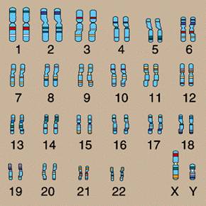
The X and Y chromosomes are called the sex chromosomes for an obvious reason – they determine the sex. Specifically:
Males have one Y chromosome and one X chromosome.
Females have two X chromosomes.
One sex chromosome comes from each parent.
Floating around the nucleus of each cell are the energy bars of the cell, known as mitochondria. Each mitochondria is composed of DNA called mitochondrial DNA or mtDNA.
You inherit your Y chromosome intact from your father, who inherited it from his father, etc., all the way back to Adam And you inherit your mtDNA intact from your mother, who inherited it from her mother, etc., all the way back to Eve. So every male should have the identical Y chromosome to Adam and everyone should have the identical mtDNA to Eve.
But mistakes do happen, and sometimes a mutation occurs when a Y chromosome is passed from father to son, or when mtDNA is passed from mother to child. It is these mistakes that allow us to categorize individuals, and to determine the most recent common ancestor to a pair of individuals.
So now we see how to use DNA to determine the descendants of our father’s father’s father’s father’s father and our mother’s mother’s mother’s mother’s mother. But what about the descendants of our other 30 great great great grandparents? That’s where the autosomes are useful.
2. IT STARTED WITH MENDEL
Gregor Mendel is credited as the father of genetics. He performed his now-famous pea experiments in Austria almost 200 years ago. By doing selective cross breeding of pea plants and observing the statistical results of the offspring, he was able to postulate two laws. These laws are the following:
a. Mendel’s First Law: Segregation of Characteristics
Despite its non-descript (and perhaps misleading) title, what this law says is “you inherit one gene randomly from each parent.” Let’s consider a gene, such as eye color. Your father has two genes for eye color. Let’s assume he has one gene for light-colored eyes and one for dark-colored eyes. You inherit one of those two genes, but which one you get is completely random. You might inherit the light-colored gene and your sibling might inherit the same or the other gene.
As a side remark, when the two genes for a trait contradict each other (as was the case for your father who had one light gene and one dark gene), one of the two genes dominates. It is called the dominant gene and the other is called the recessive gene. In the case of eye color, the dark gene is dominant and the light gene is recessive. A person having one dominant gene and one recessive gene for a particular trait is said to be hybrid for that trait.
b. Mendel’s Second Law: Independent Assortment
Again we have a law with a seemingly meaningless title, but it says something very important. It says “you inherit each gene independently of the other genes.” That is, if you inherited your father’s gene for light-colored eyes, you still have a 50:50 chance as to which of his two genes for hair color you will inherit.
c. Examples
Example 1: Let’s consider cats and the gene for determining fur color. Let us assume that the fur can be either brown or white, with brown being dominant. That is, if a cat had one gene for brown fur and one for white fur, the cat would have brown fur.
Let’s designate the gene for brown fur as “B” (upper case because it is the dominant gene) and the gene for white fur as “b” (lower case because it is the recessive gene). It might have seemed more logical to use “w” for white rather than “b”. But by using “B” and “b”, we are making it clear that they are for the same trait, and we are also making it clear which of the two is dominant.
Let’s start with two parent cats, each of which have both a dominant and recessive gene for fur color. That is, they both have one “B” gene and one “b” gene. Of course the parents could have had other combinations of genes, but focusing on these specific parents will make the analysis simple.
Mendel’s first law says that these genes are inherited randomly. In other words, each kitten has an equal chance of getting a “B” or a “b” from its father, and of getting a “B” or a “b” from its mother. This is illustrated in the diagram below.
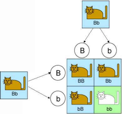
So there are four equally-likely types of kittens that could result from this mating. One type will inherit a “b” from both parents and will have white fur. The kittens in the other three types will all have brown fur because they will be either pure brown or hybrid. And this is borne out by experiments. Indeed 25% of the offspring in such experiments have brown fur.
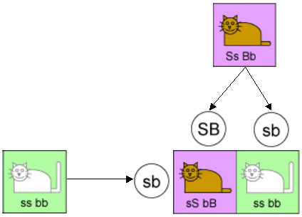
Example 2: Now consider Mendel’s second law, which has to do with more than one pair of genes. So let’s add the gene for determining tail length. Assume that the tail can be either short or long, and that short is dominant. So we will designate the gene for short tail by “S” (upper case because it is the dominant gene) and the gene for long tail by “s” (lower case). And to keep the analysis simple, we are going to start with one parent cat having all recessive genes (“s”, “s”, “b”, “b”) and the other being hybrid for each trait (“S”, “s”, “B”, “b”).
Mendel’s second law says that each gene is inherited independently of the other genes. So 25% of the time a kitten will inherit “S” and “B” from the hybrid parent, 25% of the time “S” and “b”, 25% of the time “s” and “B”, and 25% of the time “s” and “b”. From the other parent it will always inherit “s” and “b” because that is all that that parent has to offer. This is illustrated in the following diagram.
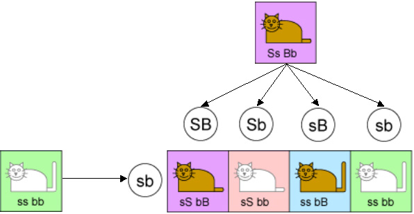
Of the four equally likely types of kittens in this case, we would expect one to be short-tailed brown, one to be short-tailed white, one to be long-tailed brown, and one to be long-tailed white. The ratio should be 25:25:25:25. And for many pairs of genes, the experiments produced offspring in exactly this ratio.
d. Mendel’s Mistake
However Mendel’s second law is not quite correct. And the reason Mendel was wrong is because he didn’t know about chromosomes – they weren’t discovered until after his death. So he didn’t know that genes are actually contained in packets (the chromosomes), and they remained together in the same packet when inherited from parent to child.
Genes that are on the same chromosome would not be inherited independently. Consider the previous example, but now assume that the fur-color gene and tail-length gene are on the same chromosome. And assume that the hybrid parent has his “S” and “B” genes on one chromosome of a chromosome pair (recall that chromosomes come in pairs) and his “s” and “b” genes on the other chromosome of the pair. In this case that parent will pass “S” and “B” to a kitten 50% of the time, and “s” and “b” the other 50%. That parent will never pass “S” and “b”, nor will it ever pass “s” and “B”. This is illustrated by the following diagram.
In this case we should expect to see 50% short-tailed browns, and 50% long-tailed whites. In theory, this is what should happen for a pair of genes on the same chromosome. But when experiments were done, the results were slightly different. What was observed was something like:
49% short-tailed brown
1% long-tailed brown
1% short-tailed white
49% long-tailed white
For genes on different chromosomes we indeed get the 25:25:25:25 ratio that the theory predicts. But for genes on the same chromosome we don’t quite get the 50:50 ratio but get something very close to it instead. There must be something else going on here. And there is, but I need to introduce some biology before I can explain it.
3. ALONG COME DNA AND CROSSOVER
You probably remember hearing terms like mitosis and meiosis in your high-school biology class. And you’ve probably long-since forgotten what they are all about, and perhaps you never really understood it in the first place. Maybe it was the terminology that made it so difficult to learn and/or remember.
So let me say a word about terminology. I sincerely believe that geneticists are good people. They have names like chromosome 1, chromosome 2, etc., and that makes the science of genetics relatively easy to learn.
Biologists on the other hand are elitists. They have terms like mitosis, meiosis, telephase, prophase, anaphase, and so on. I’m convinced they have done so in order to prevent lay people from understanding their science. To simplify things, I will use my own, more intuitive terminology when I explain the concepts.
Let’s start with the seemingly-meaningless terms – mitosis and meiosis. Both of these have to do with cell division, but they are for two very different purposes. The first is a means of cell duplication so that the body can replace cells that were lost due to attrition. The second is cell division for the purposes of reproduction. So I will refer to the two process by my more descriptive terms of “cell duplication” and “reproduction.” But I’ll keep the biologists names in parenthesis so that those who understand it can follow my description.
a. Cell Duplication (Mitosis)
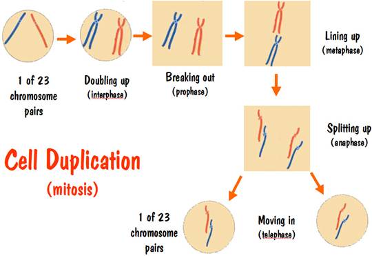
To follow the story of what happens during cell duplication, let’s look at a single chromosome pair. The same thing happens with all the chromosome pairs, but it’s much easier to focus on just two chromosomes than on 46. Let’s pretend we are watching the chromosome 7 pair. There’s nothing special about number 7 – I just needed a pair to use.
Initially all the chromosomes are inside the cell membrane, and the cell contains two copies of chromosome number 7. Let’s color these two number 7 chromosomes with different colors so we can follow them during the duplication process. We’ll color one red and the other blue (see the CELL DUPLICATION diagram below).
When duplication starts, the first thing that happens is that the chromosomes double up. That is, the blue number 7 chromosome becomes two blue number 7 chromosomes. These two blue number 7 chromosomes are identical to each other – they contain the exact same DNA sequence of base pairs. And the same thing happens for the red number 7 chromosome. But recall that the blue number 7 chromosome has a different DNA sequence than the red number 7 chromosome.
In this doubling-up phase, the two blue (or two red) chromosomes are connected at the neck and appear as an X shape. This is the only time that chromosomes are actually visible, and is the reason that you often see chromosomes drawn as an X shape (it has nothing to do with the X chromosome).
Up until now the doubled-up chromosomes are still inside the cell membrane. But the next thing that happens is that the chromosomes break out and the cell membrane vanishes. They are now free spirits, so to speak.
Next the free-spirit doubled chromosomes line up in a plane. Of course it’s hard to visualize a plane when we are focusing on just two doubled-up chromosomes – the red number 7 and the blue number 7. But remember that all the other chromosome pairs are doing the same thing.
After the chromosomes line up, they split up. That is, the two blue number 7 chromosomes that were connected at the neck now break apart. And the same for the two red number 7 chromosomes. We now have four free spirits – two reds and two blues.
After the splitting-up phase comes the moving-in phase. One of the red strands pairs up with one of the blue strands, and they take up residence together in a new cell membrane. And the same thing happens with the other red strand and the other blue strand.
Note that we started with a cell having one red strand and one blue strand, and we ended with two cells, each having one red strand and one blue strand. And the new red and blue strands have the identical DNA sequence to the original red and blue strand. The two new cells are DNA identical to the original cell and to each other.
b. Reproduction (Meiosis)
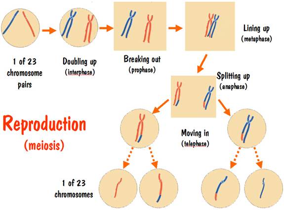
The purpose of the reproduction process is to make cells that form the seed for the next generation. For a male the seed is a sperm cell, and for a female it is an egg cell.
The reproduction process starts off similar to the cell duplication process. The chromosomes double up, break out, and line up. But something strange happens when they line up. The two number 7 doubled-up chromosomes (one red, one blue) trip over each other. Their feet get tangled up, and one of the strands of the blue pair might wind up with the foot of one of the strands of the red pair, and vice versa. This is referred to as crossover.
Next they split up, but the chromosome pairs don’t separate at this time – instead the red pair separates from the blue pair.
Following the split-up, the two red strands (still connected at the neck) move in together inside a new cell membrane, and the same for the two blue strands. But one of the red strands has a blue foot, and one of the blue strands has a red foot.
And finally, in a few more steps the doubled-up red chromosome breaks out of the cell membrane, splits into two red strands and each moves into a new cell membrane. Same of course happens to the blue chromosome. So what started off as a cell with one red strand and one blue strand for chromosome 7 winds up with four cells -- two having a single red strand and two having a single blue strand. These are the seed cells for the next generation.
The reproduction process is illustrated in the following diagram.
c. Probability of Crossover
In an ideal world, the four seed cells that were created during the reproduction process would have two complete red strands and two complete blue strands. But in the real world crossover occurs, and some red winds up on a blue strand and vice versa.
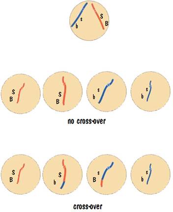
Let’s take a careful look at the chromosome that contains the fur-color and tail-size genes of the previous example. Assume that before reproduction started, one of the red strands contained the genes “S” and “B”, and the other contained the genes “s” and “b”. Furthermore let us assume that crossover for this chromosome occurs 4% of the time, and that when it does occur, the “S” and “B” gene get separated.
So how many kittens of the different combinations do we get? Let’s do 100 matings. In each mating the parent will produce 4 seed cells. (We are going to focus on just one of the parents.) There will be no crossover 96 times, so we will have 96 + 96 seed cells with “S” and “B”, and 96+96 seed cells with “s” and “b”. There will be crossover 4 times, so we will have 4 more cells with “S” and “B”, 4 more with “s” and “b”, 4 with “S” and “b”, and 4 with “s” and “B”. This is illustrated in the following diagram.
The outcome of the 100 matings is:
“S” and “B”: 96 + 96 + 4 = 196 (49%)
“s” and “b”: 96+96+4 = 196 (49%)
“S” and “b”: 4 (1%)
“s” and “B”: 4 (1%)
Note that these were the ratios that we observed when we did the cat matings but we couldn’t explain it. Now we realize that the 1% short-tailed brown and the 1% long-tailed white were due to crossover separating the genes, and the separation must have occurred 4% of the time.
So the frequency of separation is an important number. The greater the distance between two genes along the chromosome, the greater is the frequency of separation. In essence, we can measure distances along the chromosome in terms of frequency of separation. Instead of getting a distance in feet or in meters, we are getting it in percents. That might sound a bit strange, but we are all familiar with another case in which we measure distance in terms of something that is not a unit of distance. Specifically we measure the distance between two heavenly bodies not in miles but in the amount of time that it takes light to travel between them (the earth is 8 light-minutes from the sun, the nearest star to the sun is 4 light-years away).
In our example, we say that the distance between the tail-size gene and the fur-color gene is 4 because there is a 4% frequency of separation between them. But 4 what? We need to have a term for this new unit of distance. Let’s see how units of measure are named, and then we won’t be so surprised to discover what name was chosen for this new unit.
d. Naming Units of Measure
In the system of measure used in the United States, we measure small distances in inches. But there is no Mr. Inch. On the other hand, we measure units of power in watts, and there is a James Watt. There is also a Heinrich Hertz, and his name was given to the unit of frequency (equivalent to cycles per second). And there is even an Oliver Smoot, but I wonder how many of you know what a smoot is.
A smoot is the unit of distance used to measure the Harvard Bridge that is alongside MIT. Back in the 1950s, one of the MIT fraternities decided they were going to measure the bridge, and they would do so using a pledge named Oliver Smoot. Smoot would repeatedly lie on the bridge, head to toe, and one of the other pledges would paint the smoot markers. These smoot markers have now become a legend on the Harvard Bridge, and each time the bridge is repainted they are careful to repaint the smoot markers as well. And when there is an accident on the bridge, the police note its location by giving the smoot marker.
Well if we can have a watt, and a hertz, and even a smoot, we can certainly have a morgan. Thomas Hunt Morgan was a geneticist whose work involved the frequency of separation of genes. So his name became used as the measure of distance along a chromosome related to a certain frequency of separation. There is no such thing as 1 morgan, but 1/100th of a morgan (or 1 centimorgan) is the distance along a chromosome having a 1% frequency of separation. This distance varies from chromosome to chromosome, and might even vary along a chromosome. But on the average, 1 centimorgan is approximately 100 base pairs.
4. IT’S ALL ABOUT CENTIMORGANS
Now that we have centimorgans, let’s see what can we do with them. Here are three things that have been done with centimorgans:
Mapping the genome
Finding your ethnicity
Determining your cousins
We will examine each of these
a. Mapping the Genome
Mapping the human genome refers to determining which genes are on which chromosome, and where each is on the chromosome. The classic way of doing this is by a physical mapping using advanced biology techniques. But a more modern way is by using frequencies of separation, and for that we will use the centimorgans.
The way this is done is to make a very large list of traits, with each trait corresponding to a gene. For each pair of traits, determine the percent of the time that the two traits get separated (by observing the results of numerous matings). This is the distance in centimorgans between them. Once we know the centimorgans between each pair of traits, we can make a chart. For example, we might have the following chart for traits w, x, y, and z.
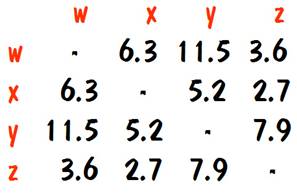
It’s not obvious at first, but if we study the number in the chart carefully we can see that the only way this can be so is if the genes for the traits are ordered along the chromosome in the sequence W-Z-X-Y. Furthermore, the distance between the genes must be:
W to Z: 3.6 centimorgans
Z to X: 2.7 centimorgans
X to Y: 5.2 centimorgans
b. Finding Your Ethnicity
Recall that the numbered chromosomes 1 to 22 are called autosomes. Due to crossover, the autosomes are not inherited intact but rather are a shuffling of the chromosome pairs from each parent. This is not true of the X chromosome when passed down from the father, nor is it true of the Y.
So DNA from all your ancestors, going all the way back, is present in the autosomes. That means that testing of the autosomal DNA can give you some statistics on your mix of ancestors.
For example, the results of an autosomal test might say that you are 50% European, 25% East Asian, 12.5% Sub-Saharan African, and 12.5% Native American. That could mean that one of your parents was 100% European, and the other was a mixture of 50% East Asian, 25% Sub-Saharan African, and 25% Native American.
That mixed parent could have one parent who was 100% East Asian and the other who was a mixture of 50% Sub-Saharan African and 50% Native American. And the latter could have one parent who was 100% Sub-Saharan African and 100% Native American (that must be the Indian Princess that we all hope to find in our family trees). This is illustrated in the following diagram.
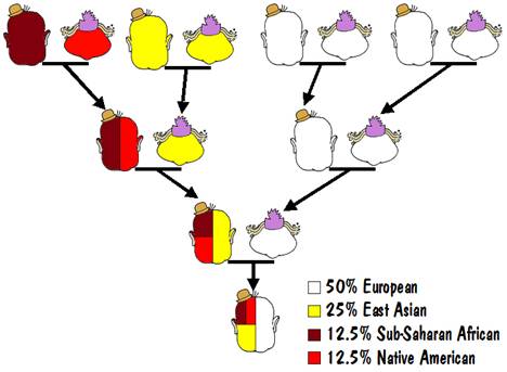
That’s not the only way it could have happened but it is the most likely. Another way would be that instead of having one parent that was 100% European, you had 50% European in both of your parents.
It should be mentioned that the percentages obtained from such autosomal testing are not very reliable. It requires a good estimate of the DNA sequences of various populations, and even small errors in these estimates can result in large errors for estimating the mixture.
c. Determining Your Cousins
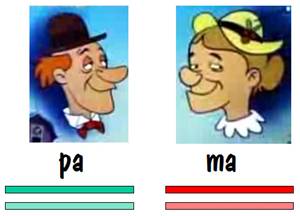
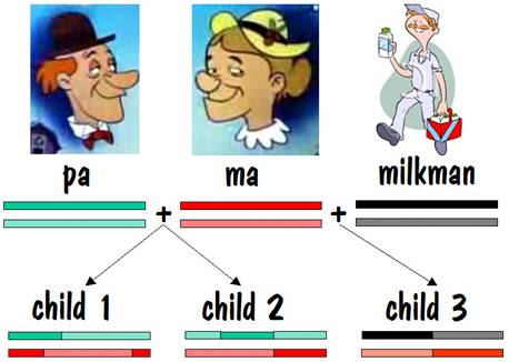
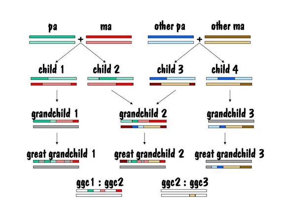
Let’s start our story with pa and ma, and we’ll follow their autosomes. We’ll focus on just one chromosome pair (number 7), but the same story applies to all the other autosomes as well.
To keep track of which chromosome is which, we’ll paint pa’s two number 7 chromosomes green, and we’ll paint ma’s red. But we’ll use different shades of red and green so that we can distinguish between each chromosome of the pair. This is shown in the diagram below.
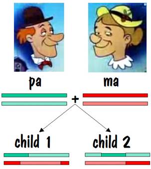
Pa and ma decided to raise a family. They had two children, and each child received one number 7 chromosome from pa and the other from ma. But the chromosomes they received contained crossover, so they were a mixture of pa’s two number 7s and ma’s two number 7s. This is shown by the alternating light and dark red or light and dark green in the two children’s number 7 chromosomes in the figure below.
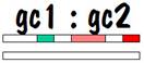
Now we can compare the chromosome map of child 1 and child 2 to see where they have common areas, and how long (in centimorgans) these common areas are. The result of the comparison is shown in the following diagram, where the white areas indicate no commonality and the colored areas indicate common areas.
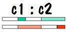
Siblings can be recognized because they have long stretches of common areas on both of their number 7 chromosomes. Of course how long is “long” is determined by statistical analysis. The testing laboratories have supposedly done enough tests of known siblings, and of known non-siblings to allow them to come up with yardsticks (or should I say “centimorgan sticks”) to distinguish between them.
Ma liked milk, and every Thursday a milkman came and delivered the milk. Nine months after the deliveries started, ma had another child. That child’s number 7 chromosome breakdown is shown below.
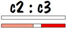
If we compare the common areas for child 3 with child 2, we will find no common areas on one of the number 7 chromosomes, and a fair amount of common area on the other. In fact, the length of the common area on the second number 7 chromosome is comparable to the length of common area found for siblings on both number 7 chromosomes. This is the identifying mark of a half sibling.
The common areas between child 2 and child 3 are shown in the figure below.
Then child 1 and child 2 each present ma and pa with a grandchild. The chromosome map for each of these two grandchildren is shown below.
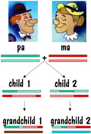
If we compare grandchild 1 with grandchild 2, we see that they have common areas on one of their number 7 chromosomes, although the length of these common areas is less than it was when we compared siblings. Furthermore, they have nothing in common on their other number 7 chromosome. This looks similar to the half-sibling case, except the lengths of the common areas are shorter. So this is the identifying mark of first cousins. The figure below shows the common areas between grandchild 1 and grandchild 2.
The reason that there is no common area on one of the number 7 chromosomes is because the spouse of child 1 and the spouse of child 2 are most likely not related. Of course there is a chance that child 1 and child 2, who were siblings, married a pair of siblings (it’s perfectly proper -- I have a few instances of this in my own family). In that case, there would be commonality on both of the number 7 chromosomes for grandchild 1 and grandchild 2. This is similar to the sibling picture, but the way we would know that we were dealing with first cousins and not siblings is that the length of the common areas (in centimorgans) is less.
If we can trust the statisticians in their assessment of what the common length is as we go further and further down the generations, we have a method of determining the relationship between two people. But we will need other information to know how they are related. That is, this test can tell you that two people are first cousins, but it won’t tell you if the relationship is through their maternal grandparents, their paternal grandparents, or some mixture thereof . The test is truly looking at all your ancestral lines, but it can’t tell you which one it found the match on.
Of course the test gets less and less reliable as more generations are involved. So the test could probably say with a high degree of certainty that two people are siblings, but with less certainty that they are fourth cousins twice removed.
d. Which cousin is it?
It is possible to use the preceding results to determine exactly how two people are related, but it's going to cost a lot more. The trick is to first identify which segment of a person's DNA came from which ancestor. Having done that, the common ancestor between two here-to-fore unrelated people is the ancestor from whom each of the two people received the matching sequence of DNA.
So how do we identify the ancestor that contributed to each segment of DNA? Let's take an example. Look at the common areas between grandchild 1 and grandchild 2 (first cousins) above. We see that they have three matching segments on their upper number 7 chromosome. And since we already know that these two people are the grandchildren of ma and pa above, we know that the three matching segments came from ma and pa. Of course the entire upper number 7 chromosome would have had to come from ma and pa as well, but we don't know that from the comparison of these two grandchildren. If we had more grandchildren of ma and pa to compare with, we might be able to determine that. And of course none of these first cousins would have any segments from ma and pa on their lower number 7 chromosome -- that chromosome came from their other set of grandparents.
Now let's compare children of grandchild 1 to children of grandchild 2 (second cousins, all great grandchildren of ma and pa). See the figure below. In this case the lengths of the matching areas are smaller. The matching areas are the DNA received from ma and pa and cover only about half of the upper chromosome 7, the rest of upper chromosome 7 and all of lower chromosome 7 comes from three other pairs of great grandparents.
So by testing enough of your known first cousins, known second cousins, etc. from all sides of your family, you can eventually determine which of your ancestors contributed to which portion of your DNA. But this means testing an awful lot of your relatives, which is why I said that this was going to be costly.
5. MORE ABOUT CHROMOSOME INHERITANCE
a. Autosomal inheritance and the 50% rule
There are 44 autosomes, numbered in pairs from 1 to 22. Rather than talking about all 22 pairs, we will focus on just one pair for simplicity, namely autosomal pair #7. Of course what we say here applies to the other 21 pairs as well.
A child inherits exactly 50% of his autosomal DNA from each parent. The reason is that the child received one #7 from his mother and one #7 from his father. Looking back one more generation, the child inherits approximately 25% of his autosomal DNA from each grandparent.
Let's see why the breakdown from each grandparent is approximate and not exact. Each paternal grandparent passes a single #7 chromosome to the father. So the father has one #7 that comes from the paternal grandfather and one that comes from the paternal grandmother. But when the father passes a #7 to the child, he does so by first shuffling his two #7s together. This shuffling does not take an equal distribution from each of the father's #7 autosomes, resulting in the distribution in the child being approximate and not exact. The same is true for the #7 chromosome from the maternal grandparents. This is illustrated in the figure below.
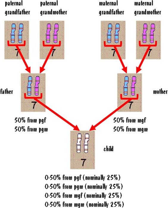
Although the 25% numbers are approximate, the actual values will usually be close to that. You might see 24:26:28:22 for example. But it would be highly unlikely that you would see radical deviations from 25%.
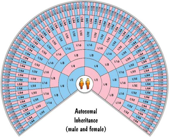
So autosomal inheritance follows the 50% rule exactly for the lowest generation and reliably for generations above that. This can be shown graphically on the family-tree fan chart below. Each ring on the chart corresponds to a generation and each cell corresponds to an ancestor. The colors of the cells indicate gender (blue for males, pink for females). The numbers in each cell correspond to the fraction of DNA that the child inherits from that ancestor.
b. Y chromosome inheritance
The Y chromosome gets passed from the father to the son. The mother doesn't have a Y chromosome, so the son gets exactly 100% of his Y-chromosome DNA from his father. And that 100% inheritance is continued all the way up the paternal line, and will be exact no matter how far back you go. That means that a male child will inherit exactly 100% of his Y-chromosome DNA from his great-great-great...grandfather. This is shown on the next fan chart.
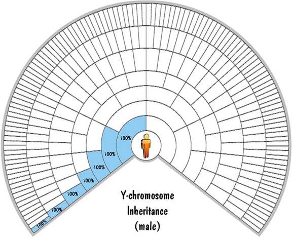
What about the Y-chromosome inheritance rule for a female child? OK, that was a trick question -- a female doesn't have any Y chromosomes.
c. X chromosome inheritance
The mother has two X chromosomes which get shuffled together and passed to the child. The father has one X chromosome and one Y chromosome. He passes one of those unshuffled to his offspring. If he passes the Y chromosome, the child is male. And if he passes the X chromosome, the child is female. So a male child inherits exactly 100% of his X-chromosome DNA from his mother. And a female child inherits exactly 50% of her X-chromosome DNA from each parent.
This is illustrated in the fan charts by the fact that each blue cell (a male) inherits all his X-chromosome DNA from his pink (female) parent on the next outer ring and none from his blue (male) parent. Also each pink cell (female) inherits half of her X-chromosome DNA from each parent. For the first generation, this 50% rule is exact. But for generations beyond that, not only is it approximate (due to shuffling), but it is very unreliable. Unlike the autosomal inheritance where the values were close to the values shown in the chart, for the X-chromosome case the values can (and do) range from zero to twice the value shown.
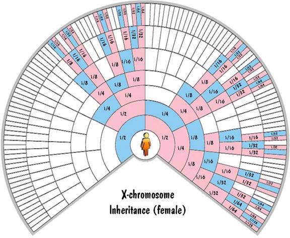
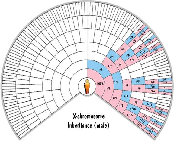
These fan charts make it clear that the inheritance pattern of the X chromosome is very complex (when compared to autosomes or to Y chromosome). There are "blackout" regions on the chart corresponding to ancestors that contribute no X-chromosome DNA. For those that do contribute, the amount of the contribution of ancestors on the same ring differs widely. And the amount of contribution shown on the chart could be highly inaccurate due to the unreliability of the 50% rule. For these reasons, you don't hear much about using X-chromosome DNA to trace your genealogy.
Blaine Bettinger was the first to use fan charts to show X-chromosome inheritance. The charts shown here extend the concept to the autosomes and the Y chromosome as well.
6. SUMMARY
The previous paper showed how to trace the direct male lineage (by using the Y chromosome) and the direct female lineage (by using mtDNA). But those methods tell nothing about all the branches in between.
The current paper shows how to use autosomes to learn something about these other lines. It’s all based on Mendel’s error in not realizing that the genes are on chromosomes and are therefore not always inherited independently of each other. Furthermore, due to crossover, the chromosomes don’t stay intact, and long segments from one chromosome of a pair are interspersed with long segments from the other chromosome of the pair. The length of these segments (measured in centimorgans), and the commonality of these segments among different people, can give information about ethnicities and relationships.
There are four significant DNA tests that are being used for genealogy purposes. Here is a summary and comparison of each. The term “recent ancestors” refers to ancestors within the last few generations, whereas “early ancestors” refers to ancestors who lived tens of thousands of years ago.
a. Y-Chromosome Testing
For males only
Traces direct male lines
Finds both recent and deep common ancestors
b. Mitochondrial DNA Testing
For both males and females
Traces direct female lines
Finds mostly deep common ancestors
c. Autosomal Ethnicity
Testing
For both males and females
Traces all lines
High error rate
d. Autosomal Cousin Testing
For both males and females
Traces all lines
Finds descendants of recent ancestors